Detection of Genetic Variants
There are many open-source tools available that enable researchers to perform variant detection from HiC data. We aim to hightlight the tools and commands we use here at Cantata Bio call features. This is not a comprenisve list, nor do we own or manage any of the tools listed below. Please refer to their source document pages for more information or for help in trouble shooting the use of these tools. For each analysis performed below we provide, a link to the tool repo, the input file, the example command, and an example output for you to check your results against.
Example input files (.mcool, .hic, or bam files)
Structural Variants
Recommended Software
hic_breakfinder https://github.com/dixonlab/hic_breakfinder
Example Command
./hic_breakfinder --bam-file K562.bam --exp-file-inter inter_expect_1Mb.hg38.txt --exp-file-intra intra_expect_100kb.hg38.txt --name hic_breakfinder/K562
Example Output(s)
Example
breaks filefile
Interpretation of Structural Variant Results
hic_breakfinder produces a number of results at various resolutions (10Kb, 100Kb, 1Mb), as well as a merged result file containing the deduplicated merged results from all three resolutions. The results file takes the form of a modified bedpe file, which contains two chromosomal positions. For example:
score |
chr1 |
start1 |
start2 |
strand1 |
chr2 |
start1 |
start2 |
strand2 |
|---|---|---|---|---|---|---|---|---|
2542.82 |
chr10 |
61000000 |
87000000 |
+ |
chr3 |
17000000 |
49000000 |
+ |
1212.33 |
chr12 |
22000000 |
35000000 |
- |
chr21 |
24000000 |
33000000 |
- |
1027.18 |
chr9 |
130000000 |
132000000 |
- |
chr22 |
22000000 |
24000000 |
+ |
958.968 |
chr6 |
16000000 |
48000000 |
+ |
chr16 |
78000000 |
86000000 |
+ |
875.468 |
chr9 |
130000000 |
132000000 |
+ |
chr13 |
80000000 |
109000000 |
- |
815.972 |
chr9 |
27000000 |
39000000 |
- |
chr13 |
19000000 |
47000000 |
- |
267.066 |
chr22 |
11000000 |
24000000 |
+ |
chr13 |
89000000 |
108000000 |
- |
246.015 |
chr18 |
27000000 |
28000000 |
- |
chr1 |
106000000 |
120000000 |
- |
128.247 |
chr22 |
22000000 |
24000000 |
- |
chr2 |
148000000 |
152000000 |
- |
64.0124 |
chr20 |
30000000 |
33000000 |
+ |
chr1 |
107000000 |
118000000 |
- |
The score column represents the most highly supported structural variants, and is a great place to begin investigating the most significant calls. In the next step, one may wish to visualise the structural variant at the matrix level. There are many tools available for visualizing HiC data at the matrix level. One possible solution is to use the .cool file and plot a region surrounding the two breakpoints using a plotting tool such as hicPlotMatrix from the HiCExplorer analysis suite (https://hicexplorer.readthedocs.io/en/latest/content/tools/hicPlotMatrix.html) For example, the following code can be used to plot a 1Mb window centered on each of the breakpoints:
hicPlotMatrix -m K562.mcool::/resolutions/8000 -out SV.png --region chr9:130000000-132000000 --region2 chr22:22000000-24000000
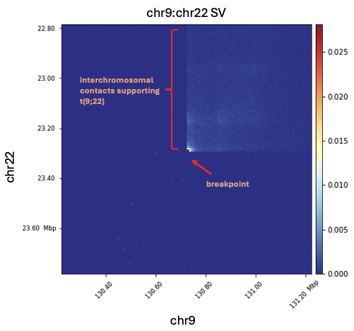
The image above depicts an translocation involving chromosome 9 and chromosome 22 (the Philadelphia translocation). The signal seen the upper right-hand quadrant represents trans chromosomal contacts between chromosome 9 and 22. The increase in signal at the center of the image indicates a strong increase in supporting ligation pairs at the SV breakpoint.
Considerations for calling SVs
Be careful when considering other structural variant callers designed for shotgun-based sequencing methods, as these many of these tools are designed to take advantage of discordant read pair information (such as Delly and Manta). As the nature of a proximity ligation library is to artificially create chimeric ligation pairs, all valid ligation pairs will be considered a “discordant” read pair, and thus attempting to use tools that rely on this information will lead to an abundance of false positive calls.
Copy Number Variation
Recommended Software
Example Command
# generate .cnr file
cnvkit.py batch K562.bam -r FlatReference.cnn -p 8 -d K562

# segment into copy number calls
cnvkit.py segment K562.cnr -o K562.cns
Example Output(s)
Example
.cnr (logR ratio)fileExample
.cns (segmentation)file
SNVs and Indels
Recommended Software
deepVariant https://github.com/google/deepvariant
Example Command
# assumes bam file and reference are in a directory named /input
docker run -v "in_dir":"/input" -v "out_dir:/output" google/deepvariant:"1.1.0" /opt/deepvariant/bin/run_deepvariant --model_type=WGS --ref=input/hg38.fa --reads=output/K562.bam --output_vcf=K562.vcf --intermediate_results_dir ./tmp --num_shards=8
Example Output(s)
Example
VCF filefile
Variant Annotation
The VCF file produced by deepVariant is fully compatible with standard variant annotation pipelines, including:
Variant Effect Predictor https://useast.ensembl.org/info/docs/tools/vep/index.html